Downloading data from Copernicus Marine Service (CMEMS) as rasters

Copernicus Marine Service, also known as Copernicus Marine Environmental Monitoring Service (CMEMS), is a distribution point for a lot of marine data produced in Europe. All Copernicus data is free, but accessing it requires you register for an account, which you should do before trying this example.

In this example, we’ll show how to use the GeoEco CMEMSARCOArray class to download time slices of a 3D chlorophyll concentration dataset and a 4D ocean temperature model as GIS-compatible raster files. CMEMSARCOArray can access most 2D, 3D, and 4D datasets published by Copernicus, providing that two of their dimensions are longitude and latitude, and the other two dimensions, if given, are time or depth. CMEMSARCOArray queries Copernicus using their Python API and downloads data using zarr. You can explore all of the Copernicus datasets here.

This example also makes use of various classes in GeoEco.Datasets, to clip the 3D and 4D grids to a geographic area of interest, to slice them into collections of 2D grids, and to create rasters for those 2D grids with GDAL.

We also have an example showing how to do this in ArcGIS with MGET’s Create Rasters for CMEMS Dataset geoprocessing tool.

Downloading chlorophyll concentration data

First, we’ll access the dataset known as Global Ocean Colour (Copernicus-GlobColour), Bio-Geo-Chemical, L4 (monthly and interpolated) from Satellite Observations (1997-ongoing). We’ve utilized this dataset frequently in our own work. We like it because it’s global, it extends back to the launch of SeaWiFS in 1997, it integrates data from whichever satellites were available during a given era, and it interpolates values for cells that were obscured by clouds or were missing data for some other reason.

Under their Data access page, you can see various datasets. We’ll use the one called cmems_obs-oc_glo_bgc-plankton_my_l4-multi-4km_P1M, which contains various phytoplankton-related variables, integrated from multiple satellites, with 4 km spatial resolution and monthly temporal resolution:

../_images/PythonDownloadingCMEMSRasters1.png

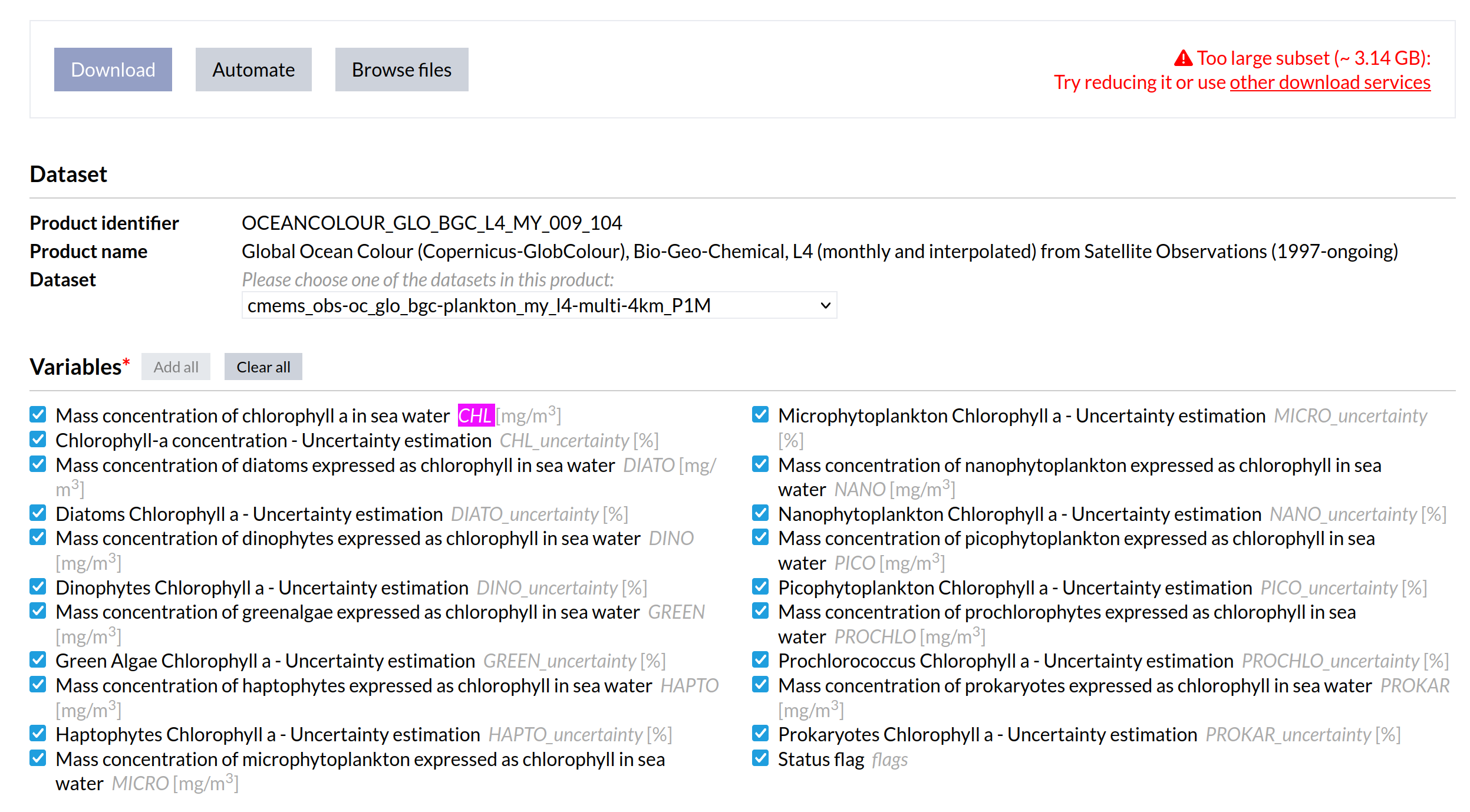
Clicking on the Form link takes you to the list of variables included in the dataset. We need to know the “short name” of the variable as it occurs in the underlying netCDF files stored in Copernicus’s cloud. We want the CHL variable, which is the mass concentration of chlorophyll a in sea water:

../_images/PythonDownloadingCMEMSRasters2.png

The code

The comments explain each part of the code.

# Edit these variables before running this script.

username='**********'                       # Replace with your Copernicus username
password='**********'                       # Replace with your Copernicus password
outputDir = '/home/jason/Development/Temp'  # Replace with your output directory

# Import GeoEco classes we'll use.

from GeoEco.Datasets.Collections import DirectoryTree
from GeoEco.Datasets.GDAL import GDALDataset
from GeoEco.Datasets.Virtual import ClippedGrid, GridSliceCollection
from GeoEco.DataProducts.CMEMS import CMEMSARCOArray
from GeoEco.Logging import Logger

# Initialize GeoEco's logging.

Logger.Initialize()

# Define a CMEMSARCOArray for Copernicus monthly GlobColour chlorophyll
# concentration, which is 3D with dimensions time, latitude, and longitude.

grid = CMEMSARCOArray(username=username,
                      password=password,
                      datasetID='cmems_obs-oc_glo_bgc-plankton_my_l4-multi-4km_P1M',
                      variableShortName='CHL')

# Clip the grid to our region of interest, the western North Atlantic in this
# example. Coordinates for CMEMSARCOArray grids are longitude (-180 to 180)
# and latitude (-90 to 90). You can adjust the coordinates to your own study
# area as desired.

grid = ClippedGrid(grid, clipBy='Map coordinates', xMin=-82, xMax=-52, yMin=25, yMax=50)

# Define a GridSliceCollection that slices the CMEMSARCOArray into a
# collection of 2D (latitude, longitude) grids. We don't say here which time
# slices we want; that comes later.

slices = GridSliceCollection(grid)

# Define a DirectoryTree that describes how we want to create the slices when
# we import them: as GDAL datasets stored in subdirectories for the Copernicus
# dataset, year, and variable short name, and named with the variable short
# name, year, and month. Store them in ERDAS IMAGINE raster format (.img). In
# order for these expressions to work, QueryableAttributes have to be defined
# for them; we can take the definitions from the GridSliceCollection.

dirTree = DirectoryTree(path=outputDir,
                        datasetType=GDALDataset,
                        pathCreationExpressions=['%(DatasetID)s',
                                                 '%(VariableShortName)s',
                                                 '%%Y',
                                                 '%(VariableShortName)s_%%Y%%m.img',],
                        queryableAttributes=slices.GetAllQueryableAttributes())

# Query the slices for datasets within a range of years and import them into
# the directory tree. We could also have used ClippedGrid above to constrain
# the time range, but I preferred to do it in the query here. Also calculate
# statistics for the rasters.

dirTree.ImportDatasets(datasets=slices.QueryDatasets('Year >= 2020 AND Year <= 2022'),
                       calculateStatistics=True)

The output

When the last line of code is executed (dirTree.ImportDatasets), this output is generated:

2024-09-17 22:42:11.543 INFO Querying Copernicus Marine Service catalogue for dataset ID "cmems_obs-oc_glo_bgc-plankton_my_l4-multi-4km_P1M".
2024-09-17 22:42:31.716 INFO Querying time slices of variable CHL of Copernicus Marine Service dataset cmems_obs-oc_glo_bgc-plankton_my_l4-multi-4km_P1M, clipped to indices yMin = 2760, yMax = 3359, xMin = 2352, xMax = 3071 for datasets matching the expression "Year >= 2020 AND Year <= 2022".
2024-09-17 22:42:31.777 INFO Query complete: 0:00:00 elapsed, 36 datasets found, 0:00:00.001703 per dataset.
2024-09-17 22:42:31.777 INFO Importing 36 datasets into directory /home/jason/Development/Temp with mode "add".
2024-09-17 22:42:31.779 INFO Checking for existing destination datasets.
2024-09-17 22:42:31.780 INFO Finished checking: 0:00:00 elapsed, 36 datasets checked, 0:00:00.000005 per dataset.
2024-09-17 22:42:31.780 INFO 0 destination datasets already exist. Importing 36 datasets.
2024-09-17 22:42:51.656 INFO Import complete: 0:00:19 elapsed, 36 datasets imported, 0:00:00.552107 per dataset.

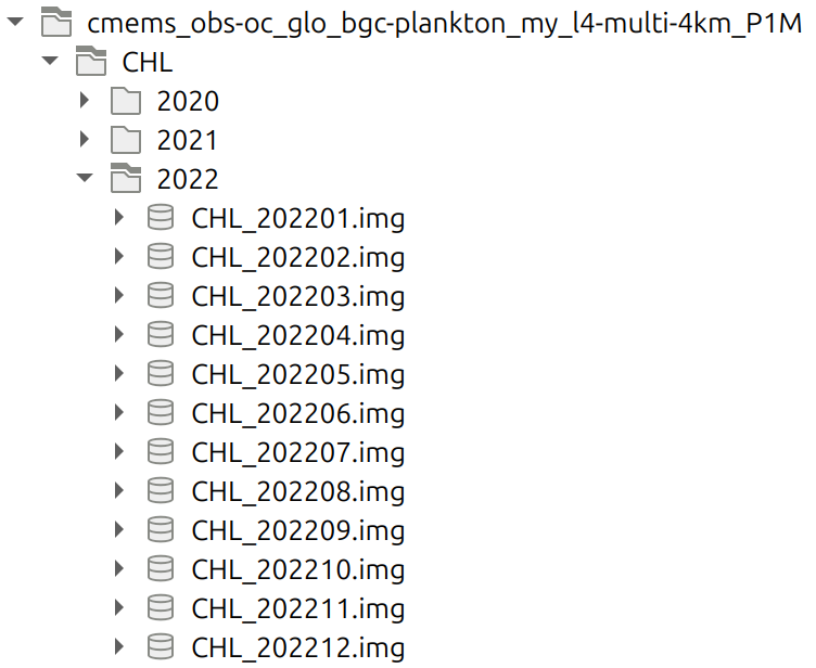
The resulting directory structure looks like this in QGIS:

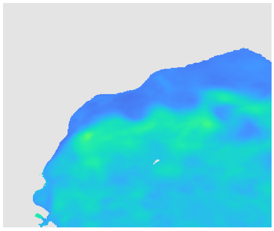
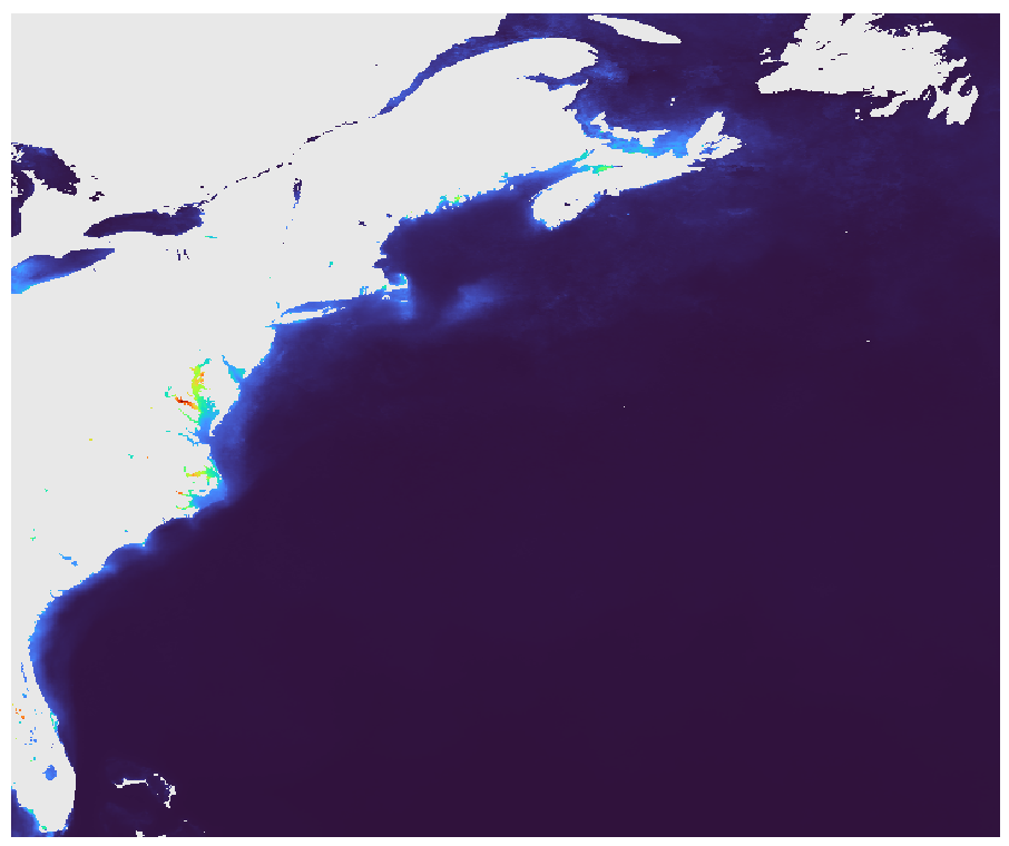
../_images/PythonDownloadingCMEMSRasters3.png

Here’s one image symbolized with the “turbo” color ramp:

../_images/PythonDownloadingCMEMSRasters4.png

Downloading 4D ocean model temperature data

New, we’ll access the dataset known as Global Ocean Physics Reanalysis, a 1/12° horizontal resolution 4D ocean model with 50 depth levels, also known as GLORYS12. We like this dataset because it extends back to 1993 (roughly to the launch of TOPEX/Poseidon) and because it scored very well in an evaluation of how eight global ocean models performed for the northeast U.S. continental shelf (Castillo-Trujillo et al. 2023), a region that our lab frequently works in.

Under their Data access page, we want the cmems_mod_glo_phy_my_0.083deg_P1M-m dataset, which has a temporal resolution of 1 month, and at the time of this writing contained data ranging from 1993 to mid-2021. The corresponding _myint_ dataset contained data from mid-2021 forward, known as the “interim period”. After clicking on the Form link, we determined we wanted thetao variable, which is the sea water potential temperature.

The code

The code is very similar to the chlorophyll example above, with the main differences being:

We instantiate the CMEMSARCOArray with the parameters needed for the ocean model data instead.
We set the zMin and zMax parameters of ClippedGrid to restrict which depth levels we want.
We instantiate the DirectoryTree with pathCreationExpressions that create an additional subdirectory for depth.

# Edit these variables before running this script.

username='**********'                       # Replace with your Copernicus username
password='**********'                       # Replace with your Copernicus password
outputDir = '/home/jason/Development/Temp'  # Replace with your output directory

# Import GeoEco classes we'll use.

from GeoEco.Datasets.Collections import DirectoryTree
from GeoEco.Datasets.GDAL import GDALDataset
from GeoEco.Datasets.Virtual import ClippedGrid, GridSliceCollection
from GeoEco.DataProducts.CMEMS import CMEMSARCOArray
from GeoEco.Logging import Logger

# Initialize GeoEco's logging.

Logger.Initialize()

# Define a CMEMSARCOArray for the thetao variable of the Global Ocean Physics
# Reanalysis, which is 4D with dimensions time, depth, latitude, and
# longitude.

grid = CMEMSARCOArray(username=username,
                      password=password,
                      datasetID='cmems_mod_glo_phy_my_0.083deg_P1M-m',
                      variableShortName='thetao')

# Clip the grid to our region of interest, the western North Atlantic in this
# example. Coordinates for CMEMSARCOArray grids are longitude (-180 to 180)
# and latitude (-90 to 90). You can adjust the coordinates to your own study
# area as desired. Also clip to the depths of interest, 0 to 1000 meters in
# this example.

grid = ClippedGrid(grid, clipBy='Map coordinates', xMin=-82, xMax=-52, yMin=25, yMax=50, zMin=0, zMax=1000)

# Define a GridSliceCollection that slices the CMEMSARCOArray into a
# collection of 2D (latitude, longitude) grids. We don't say here which time
# slices we want; that comes later. We chose to constrain the depth slices
# with ClippedGrid above, but could also have done that later.

slices = GridSliceCollection(grid)

# Define a DirectoryTree that describes how we want to create the slices when
# we import them: as GDAL datasets stored in subdirectories for the Copernicus
# dataset, year, and variable short name, and named with the variable short
# name, depth, year, and month. Store them in ERDAS IMAGINE raster format
# (.img). In order for these expressions to work, QueryableAttributes have to
# be defined for them; we can take the definitions from the
# GridSliceCollection.
#
# Note that the depth levels used by the Global Ocean Physics Reanalysis
# products are not rounded to simple values like 10, 20, 50, and 100. Instead,
# they appear to use some algorithmic spacing. Reflecting this, we format the
# depth directories with two decimal digits. We also pad the depths with
# leading zeros. The 07.02f accomplishes this. We did not include depth in the
# file name, but if you wanted to do that, you could insert the depth formatter
# into the file name, something like this:
#
#     '%(VariableShortName)s_%(Depth)07.02f_%%Y%%m.img'

dirTree = DirectoryTree(path=outputDir,
                        datasetType=GDALDataset,
                        pathCreationExpressions=['%(DatasetID)s',
                                                 '%(VariableShortName)s',
                                                 'Depth_%(Depth)07.02f',
                                                 '%%Y',
                                                 '%(VariableShortName)s_%%Y%%m.img',],
                        queryableAttributes=slices.GetAllQueryableAttributes())

# Query the slices for datasets within a range of years and import them into
# the directory tree. Also calculate statistics for the rasters.

dirTree.ImportDatasets(datasets=slices.QueryDatasets('Year >= 2020 AND Year <= 2022'),
                       calculateStatistics=True)

The output

Many more rasters are created this time, because of the many depth levels:

2024-09-18 13:45:03.762 INFO Querying Copernicus Marine Service catalogue for dataset ID "cmems_mod_glo_phy_my_0.083deg_P1M-m".
2024-09-18 13:45:23.363 INFO Querying time and depth slices of variable thetao of Copernicus Marine Service dataset cmems_mod_glo_phy_my_0.083deg_P1M-m, clipped to indices zMax = 34, yMin = 1260, yMax = 1560, xMin = 1176, xMax = 1536 for datasets matching the expression "Year >= 2020 AND Year <= 2022".
2024-09-18 13:45:27.230 INFO Query complete: 0:00:03 elapsed, 630 datasets found, 0:00:00.006139 per dataset.
2024-09-18 13:45:27.231 INFO Importing 630 datasets into directory /home/jason/Development/Temp with mode "add".
2024-09-18 13:45:27.276 INFO Checking for existing destination datasets.
2024-09-18 13:45:27.279 INFO Finished checking: 0:00:00 elapsed, 630 datasets checked, 0:00:00.000005 per dataset.
2024-09-18 13:45:27.279 INFO 0 destination datasets already exist. Importing 630 datasets.
2024-09-18 13:46:27.367 INFO Import in progress: 0:01:00 elapsed, 103 datasets imported, 0:00:00.583379 per dataset, 527 remaining, estimated completion time: 09:51:34.
2024-09-18 13:51:27.333 INFO Import complete: 0:06:00 elapsed, 630 datasets imported, 0:00:00.571515 per dataset.

The resulting directory structure includes those levels:

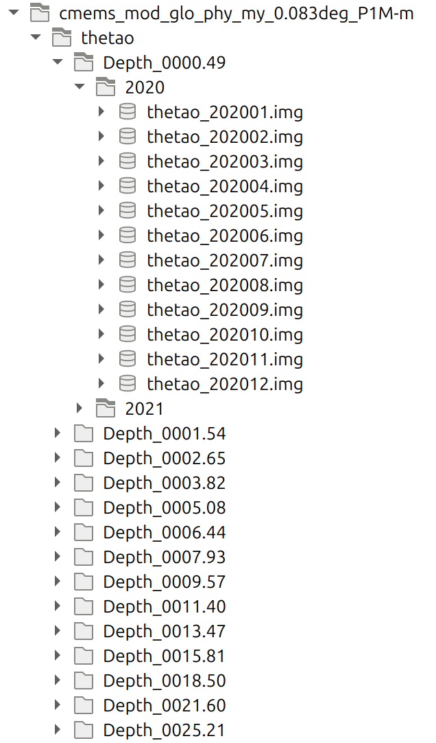
../_images/PythonDownloadingCMEMSRasters5.png

(Not all depth levels are shown in this screenshot.)

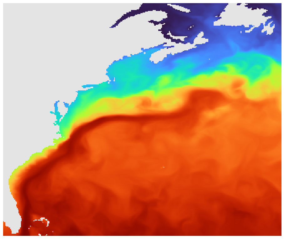
Here’s one image at the depth of 1.54 meters symbolized with the “turbo” color ramp:

../_images/PythonDownloadingCMEMSRasters6.png

Here’s the same time slice at 902.34 meters with the same color scale:

../_images/PythonDownloadingCMEMSRasters7.png